The HMM procedure in SAS Viya supports hidden Markov models (HMMs) and other models embedded with HMM. PROC HMM supports finite HMM, Poisson HMM, Gaussian HMM, Gaussian mixture HMM, the regime-switching regression model, and the regime-switching autoregression model. This post introduces Poisson HMM, the latest addition to PROC HMM in the SAS Viya 2023.03 release.
Count time series is ill-suited for most traditional time series analysis techniques, which assume that the time series values are continuously distributed. This can present unique challenges for organizations that need to model and forecast them. As a popular discrete probability distribution to handle the count time series, the Poisson distribution or the mixed Poisson distribution might not always be suitable. This is because both assume that the events occur independently of each other and at a constant rate. In time series data, however, the occurrence of an event at one point in time might be related to the occurrence of an event at another point in time, and the rates at which events occur might vary over time.
HMM is a valuable tool that can handle overdispersion and serial dependence in the data. This makes it an effective solution for modeling and forecasting count time series. We will explain how the Poisson HMM can handle count time series by modeling different states by using distinct Poisson distributions while considering the probability of transitioning between them.
What are HMMs?
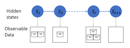
HMMs are a class of models where the distribution that generates an observation is dependent on the state of an underlying, unobserved Markov process. Figure 1 illustrates how demand varies based on the hidden state. In State 1 (S1), the demand is two units; in State 2 (S2), the demand is one unit; in State t (St), the demand is three units, and in State t+1 (St+1), the demand is zero units. Of course, you might already know the power of HMM through my blog post on the SAS Batting Lab. The Poisson HMM is a specific type of HMM where different states are modeled by using distinct Poisson distributions while considering the probability of transitioning between them.
Poisson HMM simulated example
To demonstrate the effectiveness of a certain approach, a simulated example was created in the context of the retail industry. Specifically, the example involved generating a set of count data with small, discrete values that mimicked the demand pattern of a product with a slow-moving inventory. This type of data is frequently encountered in inventory control problems, especially for items with low demand rates. The objective of this example was to illustrate the challenges associated with analyzing such data to help make inventory plans.
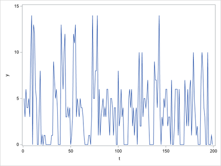
To begin with, Figure 2 displays the first 200 of the total 1000 observations of the generated time series. This gave an insight into the overall pattern of the data. Additionally, Figure 3 demonstrates that the values of the time series were discrete, ranging from 0 to 18. Moreover, it was found that 27.3% of the time series consisted of zeroes. This indicated that the time series was a count time series with a considerable number of zero values.

The mean and variance shown in Table 1 indicate there is overdispersion of the data.

Challenges
One of the challenges in model training is to determine the appropriate number of hidden states to use in the model. One approach is to search for models with different numbers of states. You can then compare their information criteria to identify the best model. In this study, we used the Akaike information criterion (AIC) to select the optimal model. After comparing the AIC values of the models with 1 to 10 states in Table 2, we found that the model with three hidden states had the smallest AIC value. So it would be the most suitable. The Poisson HMM model allows for multiple hidden states, each of which might represent times of varying customer demand.

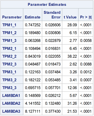
The parameter estimates shown in Table 3 reveal that the means (lambda) of the Poisson distribution for the three hidden states are 0.148569, 4.141552, and 8.127111. The state with a mean of 0.148569 is particularly effective at generating zero values in the observations. We can categorize these three states as low, normal, and high-demand states in the retail industry. This would be helpful in making inventory plans.
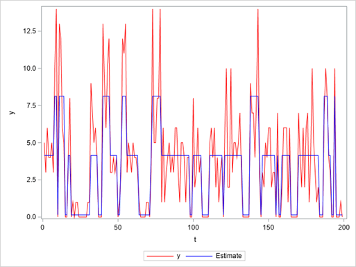
The plot in Figure 4 overlays the decoded hidden states (blue line) of the Poisson HMM onto the count time series (red line). The predominance of zero values is reflected by the troughs in the blue line, which corresponds to the low-demand state that generates mostly zeros.
The HMM procedure can also be used to forecast count time series. Table 4 shows the one-step forecast of the Poisson HMM. The state with low demand has a probability of 0.10884, the state with normal demand has a probability of 0.82668, and the state with high demand has a probability of 0.064485. The expected mean of the mixed Poisson distribution for the next period is 3.96397. The table also lists the quantiles of the predicted distribution. The 0.025 quantile equals 0, the median equals 4, and the 0.975 quantile equals 10.

Summary
In this post, we introduced the Poisson HMM. It is a useful tool for modeling discrete time series and dealing with overdispersed and serially correlated data. The HMM procedure implements a powerful technique that can estimate parameters, decode the hidden states, and forecast the series. For further information on HMMs, visit The HMM Procedure. Here you will find more types of HMMs, more algorithms, and more applications in different fields. The SAS code for this example can be downloaded from GitLab.


3 Comments
I really enjoyed this blog. I would like to replicate and potentially expand upon this example. I, however, encounter a DNS error when I try to go to the GirLab site. Assistance in this matter would be greatly appreciated.
Hi Jonathan,
The link to the SAS file is: https://gitlab.sas.com/Ji.Shen/poissonhmm_example
It is a publicly accessible link on GitLab.
Please let me know how it works.
Thanks!
Hi Jonathan,
The previous link is only accessible within the SAS organization.
I have updated a publicly accessible link: https://gitlab.com/sas1564528/poissonhmm_example
Please let me know if it doesn't work.
Thanks!